


Abstract
The detection of cyclotron resonance scattering features (CRSFs) is the only way to directly and reliably measure the magnetic field near the surface of a neutron star (NS). The broad energy coverage and large collection area of Insight-HXMT in the hard X-ray band allowed us to detect the CRSF with the highest energy known to date, reaching about 146 keV during the 2017 outburst of the first galactic pulsing ultraluminous X-ray source (pULX) Swift J0243.6+6124. During this outburst, the CRSF was only prominent close to the peak luminosity of ∼2 × 1039 erg s−1, the highest to date in any of the Galactic pulsars. The CRSF is most significant in the spin-phase region corresponding to the main pulse of the pulse profile, and its centroid energy evolves with phase from 120 to 146 keV. We identify this feature as the fundamental CRSF because no spectral feature exists at 60–70 keV. This is the first unambiguous detection of an electron CRSF from an ULX. We also estimate a surface magnetic field of ∼1.6 × 10¹³ G for Swift J0243.6+6124. Considering that the dipole magnetic field strengths, inferred from several independent estimates of magnetosphere radius, are at least an order of magnitude lower than our measurement, we argue that the detection of the highest-energy CRSF reported here unambiguously proves the presence of multipole field components close to the surface of the neutron star. Such a scenario has previously been suggested for several pulsating ULXs, including Swift J0243.6+6124, and our result represents the first direct confirmation of this scenario.
Export citation and abstract BibTeX RIS

Original content from this work may be used under the terms of the Creative Commons Attribution 4.0 licence. Any further distribution of this work must maintain attribution to the author(s) and the title of the work, journal citation and DOI.
1. Introduction
Ultraluminous X-ray (ULX) sources are bright X-ray sources with apparent luminosity >1039 erg s−1, which is above the Eddington limit of a 10 M⊙ black hole (BH) (Kaaret et al. 2017). X-ray pulsations detected in ULX sources such as M82 X-2 (Bachetti et al. 2014), NGC 7793 P13 (Fürst et al. 2016; Israel et al. 2017a), NGC 5907 ULX1 (Israel et al. 2017b), NGC 300 ULX1 (Carpano et al. 2018), and RX J0209.6-7427 (Chandra et al. 2020) indicate that some, or even most ULXs are accreting neutron stars (NSs) with a strong magnetic field. A potential detection of a proton CRSF at 4.5 keV in the ULX source M51 ULX-8 implies a magnetar-like field ∼1015 G (Brightman et al. 2018). Such a strong dipole magnetic field prevents the spherization by radiation in its accretion disk even at luminosities >1041 erg s−1 (Basko & Sunyaev 1976).
Alternative estimations of the dipole magnetic fields of NSs can be made from the accretion torque, which has a close connection with the inner edge of the accretion disk influenced by the NS's magnetosphere. However, different accretion torque models might give large measurement disparities of magnetic fields in the range of 1010–1015 G (Chen et al. 2021). The estimated lower values (<1013 G) in these pulsating ULXs will make them essentially indistinguishable from Be X-ray pulsars, with the exception of their higher luminosities, which have been proposed to be a consequence of the strong beaming effect by the disk outflow, when the disk is spherized by radiation pressure (King et al. 2001; King 2009; King & Lasota 2016; King et al. 2017; Koliopanos et al. 2017; King & Lasota 2019, 2020). From the relationship between the magnetic field and maximum luminosity (see Figure 5 in Mushtukov et al. 2015), it can be seen that only when the dipole magnetic field is greater than 1013 G can the maximum accretion luminosity of magnetized pulsars be significantly greater than 1039 erg s−1. However, from the first discovery of CRSF in Her X-1 to the present (Truemper et al. 1978; Staubert et al. 2019), a direct measurement of such a strong magnetic field has not been possible by observing the expected electron CRSF because of the relatively low cutoff energy of the nonthermal emission from NS ULX systems and the lack of sensitive hard X-ray coverage above about 80 keV of contemporary X-ray telescopes. Fortunately, the launch of Insight-HXMT in 2017 (Zhang et al. 2014; Zhang et al. 2020), which has a broad energy coverage and a large detection area at energies above 100 keV, changed the situation. The two previous records of the highest energy detection of CRSFs with higher than 5σ significance were also both set by Insight-HXMT—the ∼90 keV fundamental CRSF from GRO J1008–57 (Ge et al. 2020) and the ∼100 keV first harmonic of a CRSF from 1A 0535+262 (Kong et al. 2021; Kong et al. 2022)—proving that Insight-HXMT has a strong advantage in detecting high-energy CRSFs.
The transient X-ray source Swift J0243.6+6124 was discovered on 2017 October 3 by the Swift/BAT telescope at a flux level of ∼80 mCrab before it entered into a giant outburst from 2017 to 2018 (Cenko et al. 2017; Kennea et al. 2017). A 9.8 s period pulsation was detected in X-ray observations by Swift/XRT and an eccentric binary system with a ∼28 day orbital period was revealed by Fermi-GBM (Bahramian et al. 2017; Ge et al. 2017; Kennea et al. 2017; Doroshenko et al. 2018). Optical observations assigned a Be star as the companion (Kouroubatzakis et al. 2017; Kennea et al. 2017; Stanek et al. 2017; Yamanaka et al. 2017). A distance of 6.8 kpc as reported in Bailer-Jones et al. (2018) based on Gaia DR2 parallax measurements of the companion star implies that the source is the first Galactic pulsing ultraluminous X-ray source (pULX).
The magnetic field of Swift J0243.6+6124 was estimated in various manners, yet no consensus has been reached on its surface magnetic field strength. Pure timing analyses based on Insight-HXMT's high-cadence observations reveal two typical luminosities, around which the source is believed to have experienced transitions of different emission modes at the magnetic pole and different accretion modes on the disk (Doroshenko et al. 2020b), implying a dipole surface magnetic field of ∼1012–1013 G and nontransition to the propeller state in quiescence. In particular, the nondetection of the transition allowed Tsygankov et al. (2018) to put an upper limit of ∼6 × 10¹² G assuming propeller transition below ∼6 × 1035 erg s−1, which was further reduced to ≤3 × 10¹² G by Doroshenko et al. (2020b) based on NuSTAR detection of the pulsations down to luminosities of ∼6 × 1033 erg s−1. As discussed by Doroshenko et al. (2020b), such a low dipole magnetic field allows for a coherent interpretation of the observed spin evolution of the source during the outburst, observed power spectral density, and spectral transition to correspond to the transition of the accretion disk to the radiatively dominated state. On the other hand, the estimated critical luminosity corresponding to the onset of an accretion column appeared to be more consistent with a much stronger surface magnetic field ∼1013 G (Kong et al. 2020; Liu et al. 2022). Doroshenko et al. (2020b) suggest that it could be associated with either a smaller than expected magnetospheric radius (for a given field), or the presence of strong multipole components dominating the area close to the surface of the neutron star. Here we report our very statistically significant detections of a CRSF during the 2017 outburst of Swift J0243.6+6124 observed with Insight-HXMT when the outburst peaked at a luminosity of around 2 × 1039 erg s−1, which unambiguously supports the latter scenario. We also perform detailed phase-resolved spectral analyses, given that the appearance of CRSFs can be closely phase dependent (Harding & Daugherty 1991; Nishimura 2015).
Section 2 introduces the observations and methods of data reduction. Section 3 shows the details of the timing and spectral results. In Section 4, we discuss our results. The summary and conclusions are presented in Section 5.
2. Observations and Data Reduction
The Hard X-ray Modulation Telescope (Zhang et al. 2014; Zhang et al. 2020), named Insight-HXMT, was launched on 2017 June 15. The scientific payload includes three collimated telescopes that allow observations in a broad energy band (1−250 keV) and with a large effective area at high energies: the High Energy X-ray Telescope (HE: 5000 cm2/20–250 keV; Liu et al. 2020), the Medium Energy X-ray Telescope (ME: 952 cm2/5–30 keV; Cao et al. 2020), and the Low Energy X-ray Telescope (LE: 384 cm2/1–10 keV; Chen et al. (2020). The main fields of view (FoVs) are 1.6° × 6°, 1° × 4°, and 1.1° × 5.7° for LE, ME, and HE, respectively. Ascribed to the characteristics of the three detectors, Insight-HXMT possesses a broadband capability (1−250 keV), with a large collection area at high energy and without pileup for bright sources.
Insight-HXMT was triggered with 122 pointing exposures from 2017 Oct 7 (MJD 58033) to 2018 Feb 21 (MJD 58170), which sampled the entire outburst of Swift J0243.6+6124. The Insight-HXMT Data Analysis Software (HXMTDAS) v2.04, together with the calibration model v2.05, is used for the whole process of data reduction following the recommended screening conditions by the Insight-HXMT team. In particular, data with elevation angle (ELV) larger than 10°, geometric cutoff rigidity (COR) larger than 8 GeV, and offset for the point position smaller than 0 04 are used. In addition, data taken within 300 s of the South Atlantic Anomaly (SAA) passage outside of good time intervals identified by onboard software have been rejected. In view of the conditions of in-flight calibration (Li et al. 2020), the energy bands considered for spectral analysis are 2–10 keV for LE, 10–40 keV for ME, and 30–250 keV for HE. The backgrounds are estimated with the tools provided by the Insight-HXMT team: LEBKGMAP, MEBKGMAP, and HEBKGMAP, version 2.0.9 based on the current standard Insight-HXMT background models (Liao et al. 2020a; Guo et al. 2020; Liao et al. 2020b). We note that the uncertain calibration of an Ag emission line at ∼22 keV in the ME band will leave a narrow emission line in the phase-averaged spectrum (see the left panel in Figure 2), but it fades out due to lower statistics in the phase-resolved spectrum (see the right panel in Figure 2). Considering the current accuracy of the instrument calibration and appropriate χ2, we include 1%, 0.5%, and 0.5% systematic errors for the spectral analysis for LE, ME, and HE, respectively. The uncertainties of the spectral parameters are computed using the Markov Chain Monte Carlo (MCMC) method with a length of 10,000 and are reported at a 90% confidence level. The XSPEC v12.12.0 software package (Arnaud 1996) corresponding to heasoft v6.29 is used to perform the spectral fitting and error estimation. We utilize the ftool grppha to improve the counting statistic of the spectrum (with group minimum counts of 200) by combining 10 exposures from Nov 03 to Nov 08 in 2017 with the addspec and addrmf tasks. The flux, pulse profile, and continuum spectral shape in these 10 exposures keep stable at the outburst peak (Kong et al. 2020); it is therefore reasonable to combine them in order to search for any high-energy CRSF with the best statistics. For the HE detector, the background dominates in the high-energy band, and 200 counts per bin will ensure high confidence for the net spectrum. In Figures 2 and 4, we use "setplot rebin 30 5" for a better visual display, which does not affect the fitting result.
3. Results
3.1. Phase 2D Maps
The first and foremost step of phase-resolved analysis is to get the correct phase of each photon. After barycentric and binary-orbiting corrections, the photon arriving time is converted to the real pulsating time. The parameters of the binary orbit (T0 = 58102.97476560854, Porbit = 27.698899 days, e = 0.1029,  lt-s, ω = − 7405) are taken from the website of Fermi/GBM Accreting Pulsar Histories,
8
where the spin frequencies are available on a daily basis. With such continuous and intensive monitoring, we can fit the frequency with time by the cubic spline interpolation method. Then, the phase-coherent pulse profiles considering the pulse-period changes can be derived by calculating a sequential pulse phase ϕ(t), where ϕ0 is set to 0 at t0 = 58, 027.499066 (MJD), which is the epoch of the first Fermi/GBM periodicity detection (see Sugizaki et al. 2020 for a detailed description of this method). In Figure 1, the pulse profiles folded from the background-subtracted light curves are shown in four panels with different energy bands (LE: 4.0–7.0 keV, ME: 15.0–20.0 keV, HE: 70.0–90.0 keV, 90.0–120.0 keV), and such results are similar to the results in Doroshenko et al. (2020b). From the 2D maps, we see pulse-profile transitions between different shapes at two typical luminosities as reported previously in Kong et al. (2020) and Doroshenko et al. (2020b). One is ∼ 1.5 × 1038 erg s−1 at MJD 58035 and MJD 58130, and another is ∼ 4.4 × 1038 erg s−1 at MJD 58050 and MJD 58100, probably corresponding to the onset of a pressure dominance of radiation and gas shock, respectively. At the outburst peak, the pulse profile maintains a stable bimodal structure, which allows us to do spectral analysis. The main pulse in 0.6–1.0 is above the mean count rate, and the minor pulse in 0.2–0.4 is close to or lower than the average. Such phenomena get clearer at higher energies and luminosities: At the peak of the outburst (MJD 58063), the count rate of the main pulse is four times that of the mean count rate, while it is far less than 1 for the minor peak (see the left panel in Figure 3). Figure 1 shows that the best counting statistics above 90 keV comes from the phase region 0.6–1.0 during the outburst peak (MJD 58060–58065), the data of which can be used to search for high-energy CRSFs more reliably.
lt-s, ω = − 7405) are taken from the website of Fermi/GBM Accreting Pulsar Histories,
8
where the spin frequencies are available on a daily basis. With such continuous and intensive monitoring, we can fit the frequency with time by the cubic spline interpolation method. Then, the phase-coherent pulse profiles considering the pulse-period changes can be derived by calculating a sequential pulse phase ϕ(t), where ϕ0 is set to 0 at t0 = 58, 027.499066 (MJD), which is the epoch of the first Fermi/GBM periodicity detection (see Sugizaki et al. 2020 for a detailed description of this method). In Figure 1, the pulse profiles folded from the background-subtracted light curves are shown in four panels with different energy bands (LE: 4.0–7.0 keV, ME: 15.0–20.0 keV, HE: 70.0–90.0 keV, 90.0–120.0 keV), and such results are similar to the results in Doroshenko et al. (2020b). From the 2D maps, we see pulse-profile transitions between different shapes at two typical luminosities as reported previously in Kong et al. (2020) and Doroshenko et al. (2020b). One is ∼ 1.5 × 1038 erg s−1 at MJD 58035 and MJD 58130, and another is ∼ 4.4 × 1038 erg s−1 at MJD 58050 and MJD 58100, probably corresponding to the onset of a pressure dominance of radiation and gas shock, respectively. At the outburst peak, the pulse profile maintains a stable bimodal structure, which allows us to do spectral analysis. The main pulse in 0.6–1.0 is above the mean count rate, and the minor pulse in 0.2–0.4 is close to or lower than the average. Such phenomena get clearer at higher energies and luminosities: At the peak of the outburst (MJD 58063), the count rate of the main pulse is four times that of the mean count rate, while it is far less than 1 for the minor peak (see the left panel in Figure 3). Figure 1 shows that the best counting statistics above 90 keV comes from the phase region 0.6–1.0 during the outburst peak (MJD 58060–58065), the data of which can be used to search for high-energy CRSFs more reliably.
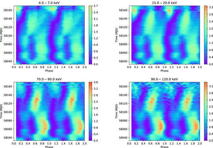
Figure 1. The two-dimensional (2D) maps describe the evolution of the pulse profile with time; the colors plot the values of the pulse values normalized by (Pulse – PulseMin)/(Average count rate – PulseMin), where PulseMin is the minimum value of the pulse intensity. The pulse profiles are folded from the background-subtracted light curves. The main pulse at phase 0.6–1.0 is above the mean count rate, and the minor peak at phase 0.2–0.4 is close to or lower than the average corresponding to the negative value for 70.0–90.0 keV and 90.0–120.0 keV.
Download figure:
Standard image High-resolution image3.2. Phase-averaged and Phase-resolved Spectrum
We combine 10 exposures in 6 days from November 3 to 8 for the high-statistic phase-resolved spectral analysis, ensuring that the exposure times of LE, ME, and HE for each phase are more than 2000 s after dividing the spectrum into 10 phase intervals. The pulse profiles in different energy bands are shown in the left panel of Figure 3. The green dashed lines show the normalized pulse value of 1, and the gray dashed lines (120–300 keV) show the normalized pulse value of 0. Significant pulse modulations are observed up to the 120–200 keV energy band with a prominent peak in phase 0.6–1.0; however, no obvious pulse modulation is visible above 200 keV.
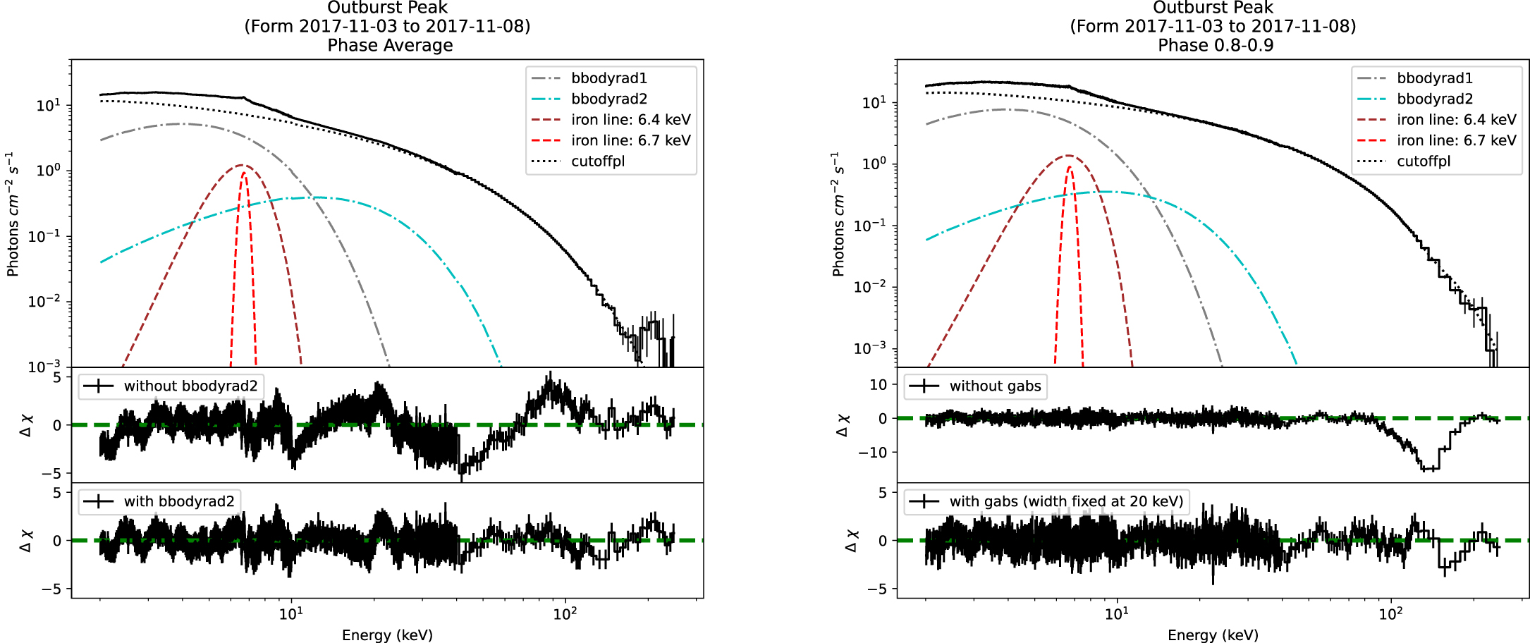
Our approach is to fit the phase-averaged spectrum and the phase-resolved spectra with the same spectral model, in order to clearly reveal the phase dependence of the spectral features. We thus first fit the phase-averaged spectrum with the model TBabs×(bbodyrad1+cutoffpl+gaussian1+gaussian2). A single blackbody with a nonthermal component model and multiple iron emission lines can well describe the phase-averaged spectra in Kong et al. (2020). The Tuebingen–Boulder ISM absorption model TBabs is taken into account (Wilms et al. 2000), and the equivalent hydrogen column density nH is fixed at 0.7 × 10²² atom cm−2, which is estimated through the Galactic H I density in the direction of Swift J0243.6+6124 (Kalberla et al. 2005). The cutoffpl is a simple nonthermal continuum with just three free parameters, normalization coefficient (CN), photon index (Γ), and exponential folding energy (Efold), respectively. We use two Gaussian models to fit multiple iron emission structures, which were reported in Jaisawal et al. (2019), and we fix the energies at 6.4 keV and 6.7 keV for neutral and ionized iron lines. The blackbody bbodyrad1 with kT1 ∼ 1.5 keV and Nbb1 ∼ 2000 was reported in Kong et al. (2020). The fitting results for the phase-averaged spectrum are shown in the left panel of Figure 2. From the residuals, adding another blackbody bbodyrad2 with high kT2 ∼ 4 keV and small Nbb2 ∼ 5 can improve the χ2 via suppressing residuals. This structure has also proved necessary in Kong et al. (2020) and Tao et al. (2019). Therefore, an extra component bbodyrad2 is added to the model to fit the phase-averaged spectrum. The lack of a significant absorption feature in the phase-averaged spectrum does not motivate us to add a CRSF.

Figure 2. We combine the observations from November 3 to November 8 in 2017 for spectral fittings. Left panel: spectral fitting and residuals of the phase-averaged spectrum. Right panel: spectral fitting and residuals of the spectrum at phase 0.8–0.9.
Download figure:
Standard image High-resolution imageNext, the same model is used for the spectral fittings of 10 different phase intervals. The fitting parameters are listed in Table 1. The spectra in phase intervals in 0.0–0.6 can be well fitted with this model, and the value of χ2 approaches the degree of freedom (DOF). In contrast, the fitting residuals of the phase intervals in 0.6–1.0 show obvious absorption features above 100 keV, which can be suppressed by introducing a Gaussian absorption model gabs; the parameters are listed in Table 1. First, the width σ of the gabs model is fixed at 20 keV, considering the low counting statistics in high-energy bands ( > 150 keV); otherwise, either the line width σ or the line energy Ecyc cannot be well constrained because these two parameters are coupled with each other. We note here that if the line width is set to another value such as 30 keV, the significance of the absorption component and the fit to the continuum spectrum do not change obviously. The fitting parameters in different phase intervals are plotted in the right panel of Figure 3. The red points denote the line energy Ecyc and absorption strength Scyc in the gabs model. We also find that Ecyc is phase dependent and varies between  keV to
  keV along the pulse phase in 0.6–1.0. The absorption feature has the maximum
  keV and largest
  (6.3σ detection significance) at the pulse peak in the phase interval. The detection significance of this CRSF varies between 6σ to 18σ at other phases. We plot the fitting and residuals in phase interval 0.8–0.9, where the residuals show a significant absorption structure above 100 keV after removing the gabs model from the overall model.

Figure 3. We combine the observations from November 3 to November 8 in 2017 for the pulse-profile analysis and the phase-resolved spectral analysis. Left panel: pulse profile evolves with energy. The background-subtracted pulse profiles are normalized by the mean count rate. The green dashed line is at 1.0, and the gray dotted line is at 0. Right panel: fitting results of the phase-resolved spectral analysis. The red points show the parameters of the CRSF.
Download figure:
Standard image High-resolution imageTable 1. Parameters of the Spectral Fitting at Different Phases
| Phase | 0.0–0.1 | 0.1–0.2 | 0.2–0.3 | 0.3–0.4 | 0.4–0.5 | 0.5–0.6 | 0.6–0.7 | 0.6–0.7 | 0.7–0.8 | 0.7–0.8 | 0.8–0.9 | 0.8–0.9 | 0.9–1.0 | 0.9–1.0 | |
|---|---|---|---|---|---|---|---|---|---|---|---|---|---|---|---|
| TBabs | nH (1022 cm−2) | 0.7 (fixed) | 0.7 (fixed) | 0.7 (fixed) | 0.7 (fixed) | 0.7 (fixed) | 0.7 (fixed) | 0.7 (fixed) | 0.7 (fixed) | 0.7 (fixed) | 0.7 (fixed) | 0.7 (fixed) | 0.7 (fixed) | 0.7 (fixed) | 0.7 (fixed) |
| gabs | Ecyc (keV) | ... | ... | ... | ... | ... | ... | ... |

| ... |

| ... |

| ... |

|
| σcyc (keV) | ... | ... | ... | ... | ... | ... | ... | 20 (fixed) | ... | 20 (fixed) | ... | 20 (fixed) | ... | 20 (fixed) | |
| Scyc | ... | ... | ... | ... | ... | ... | ... |

| ... |

| ... |

| ... |

| |
| gaussian1 | EFe1 (keV) | 6.4 (fixed) | 6.4 (fixed) | 6.4 (fixed) | 6.4 (fixed) | 6.4 (fixed) | 6.4 (fixed) | 6.4 (fixed) | 6.4 (fixed) | 6.4 (fixed) | 6.4 (fixed) | 6.4 (fixed) | 6.4 (fixed) | 6.4 (fixed) | 6.4 (fixed) |
| σFe1 (keV) |

|

|

|

|

|

|

|

|

|

|

|

|

|

| |
| norm1 |

|

|

|

|

|

|

|

|

|

|

|

|

|

| |
| gaussian2 | EFe2 (keV) | 6.7 (fixed) | 6.7 (fixed) | 6.7 (fixed) | 6.7 (fixed) | 6.7 (fixed) | 6.7 (fixed) | 6.7 (fixed) | 6.7 (fixed) | 6.7 (fixed) | 6.7 (fixed) | 6.7 (fixed) | 6.7 (fixed) | 6.7 (fixed) | 6.7 (fixed) |
| σFe2 (keV) |

|

|

|

|

|

|

|

|

|

|

|

|

|

| |
| norm2 (10−2) |

|

|

|

|

|

|

|

|

|

|

|

|

|

| |
| bbodyrad1 | kT1 (keV) |

|

|

|

|

|

|

|

|

|

|

|

|

|

|
| Nbb1 |

|

|

|

|

|

|

|

|

|

|

|

|

|

| |
| bbodyrad2 | kT2 (keV) |

|

|

|

|

|

|

|

|

|

|

|

|

|

|
| Nbb2 |

|

|

|

|

|

|

|

|

|

|

|

|

|

| |
| cutoffPL | Γ |

|

|

|

|

|

|

|

|

|

|

|

|

|

|
| Efold (keV) |

|

|

|

|

|

|

|

|

|

|

|

|

|

| |
| CN |

|

|

|

|

|

|

|

|

|

|

|

|

|

| |
| Fitting | Reduced-χ2 (dof) | 1.08 (1585) | 0.98 (1588) | 0.93 (1588) | 0.94 (1588) | 1.01 (1588) | 1.00 (1588) | 1.13 (1588) | 0.85 (1586) | 1.14 (1588) | 0.83 (1586) | 1.23 (1588) | 0.81 (1586) | 1.06 (1588) | 0.87 (1586) |
Notes. Uncertainties are reported at the 90% confidence interval and computed using MCMC (Markov Chain Monte Carlo) of length 10,000. The 1%, 0.5%, and 0.5% system errors for LE, ME, and HE have been added during spectral fittings.
Download table as: ASCIITypeset image
Now we free the width of the CRSF, which is fixed in the above spectral analyses; the results are listed in Table 2. The CRSF's width can be limited to 20−30 keV, and such a wide width of CRSF strongly disfavors the possibility of a proton cyclotron feature. We simulate 100,000 spectra using the best-fitting model parameters for phase 0.8–0.9 in Table 2 but with the CRSF excluded, and then fit these simulated spectra using the same model with and without a CRSF. The maximum Δχ2 is only 27, compared with the Δχ2 = 336 obtained by fitting to the observed spectrum; this confirms that the CRSF is detected with a high statistical significance.
Table 2. The Width of CRSF Lines Set Free to Change
| Phase | 0.6–0.7 | 0.7–0.8 | 0.8–0.9 | 0.9–1.0 | |
|---|---|---|---|---|---|
| TBabs | nH (1022 cm−2) | 0.7 (fixed) | 0.7 (fixed) | 0.7 (fixed) | 0.7 (fixed) |
| gabs | Ecyc (keV) |

|

|

|

|
| σcyc (keV) |

|

|

|

| |
| Scyc |

|

|

|

| |
| gaussian1 | EFe1 (keV) | 6.4 (fixed) | 6.4 (fixed) | 6.4 (fixed) | 6.4 (fixed) |
| σFe1 (keV) |

|

|

|

| |
| norm1 |

|

|

|

| |
| gaussian2 | EFe2 (keV) | 6.7 (fixed) | 6.7 (fixed) | 6.7 (fixed) | 6.7 (fixed) |
| σFe2 (keV) |

|

|

|

| |
| norm2 (10−2) |

|

|

|

| |
| bbodyrad1 | kT1 (keV) |

|

|

|

|
| Nbb1 |

|

|

|

| |
| bbodyrad2 | kT2 (keV) |

|

|

|

|
| Nbb2 |

|

|

|

| |
| cutoffPL | Γ |

|

|

|

|
| Efold (keV) |

|

|

|

| |
| CN |

|

|

|

| |
| Fitting | Reduced-χ2 (dof) | 0.85 (1585) | 0.82 (1585) | 0.80 (1585) | 0.86 (1585) |
Notes. Uncertainties are reported at the 90% confidence interval and computed using MCMC (Markov Chain Monte Carlo) of length 10,000. The 1%, 0.5%, and 0.5% system errors for LE, ME, and HE have been added during spectral fittings.
Download table as: ASCIITypeset image
From the phase-averaged and phase-resolved spectral fitting, the residuals do not support the addition of a 60–70 keV line during the spectral fittings. We try to add a gabs line (fixed at Ecyc = 70 keV, width = 15 keV) during the fitting and get a strength < 7 × 10⁻¹⁶, thus disfavoring the existence of such an absorption feature. This proves that the 120–146 keV absorption feature is the fundamental CRSF of Swift J0243.6+6124, which is also the highest-energy CRSF discovered so far. In Figure 4, we show the background-subtracted flux (source flux) and the systematic error of the background flux for LE, ME, and HE; their statistical errors are completely negligible. It is clear that the background uncertainties begin to dominate only above 200 keV; therefore, our detection of the CRSF is not influenced by background uncertainties.

Figure 4. The net flux of LE, ME, and HE is shown in black, red, and green points, respectively. The flux and background are obtained from the phase-resolved spectrum in phase interval 0.8–0.9. The gray line shows the systematic errors of the background flux; for the exposure time of ∼20 ks, we choose the systematic errors of 2.5%, 1.5%, and 1.5% for LE, ME, and HE, respectively, based on the HXMT background models (Liao et al. 2020a; Guo et al. 2020; Liao et al. 2020b). For such a long exposure, the statistical errors of the background flux are completely negligible.
Download figure:
Standard image High-resolution image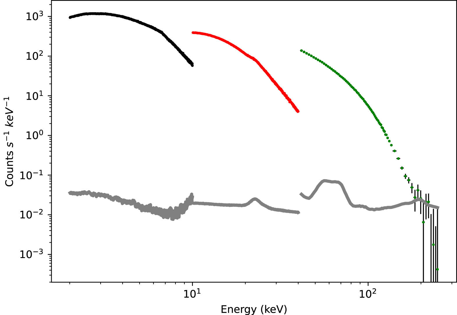
From Figure 3, the nonthermal component and two blackbody components also show significant phase-dependent structures. Γ shows a clear bimodal distribution: smaller than 1.3 during the main pulse and greater than 1.4 elsewhere, implying a harder spectrum during the main pulse. Efold increases from ∼18.6 keV to ∼30 keV when the phase changes from 0.5 to 1.0. The two thermal components are also phase dependent. The temperatures of bbodyrad1 and bbodyrad2 show a different correlation with the intensity in each phase. The negative correlation between kT2 and intensity leads to a lower temperature of ∼3 keV for the main pulse in the phase region 0.6–1.0.
In addition, we also tested whether other continuum models, such as highecut × powerlaw, NPEX, and fdcut, may influence the absorption structure. We found that the absorption structure around 140 keV is unchanged using different continuum models. We also note that when the model is NPEX, the high-temperature blackbody component (bbodyrad2) is no longer required in the fitting.
4. Discussion
We have analyzed the data from high-cadence and broadband Insight-HXMT observations of the 2017–2018 outburst of the first Galactic ULX Swift J0243.6+6124. A CRSF is discovered with high statistical significance at energies around 120–146 keV, in a period when the source stayed at a luminosity around 2 × 1039 erg s−1, far beyond the supercritical luminosity of the accretion column and the Eddington luminosity of the accreting NS. The energy of this newly detected CRSF is much higher than both the ∼90 keV fundamental CRSF of GRO J1008–57 (Ge et al. 2020) and the ∼100 keV first-harmonic CRSF of 1A 0526+261 (Kong et al. 2021, 2022); both were the previous high-energy records of CRSF detection, whose existence was firmly established for the first time by Insight-HXMT with a significance much higher than 5σ. We note that a marginal detection (absorption depth unconstrained) of the possible third CRSF harmonic at ∼128 keV was reported in the spectrum of MAXI J1409–619 (Orlandini et al. 2012). The discovery of the CRSF from Swift J0243.6+6124 reported here thus serves as the highest-energy CRSF detected so far from an NS harbored in an accreting X-ray binary system. The strength of the magnetic field can be calculated with the following relation:

where B12 is the magnetic field strength in units of 1012 G, and  is the gravitational redshift due to the NS mass and height of the line-forming region (rcyc). n is the number of the Landau level involved: e.g., n = 1 for the fundamental line and n ≥ 2 for its harmonics. The above equation assumes that the absorption takes place at the NS surface. However, in reality, the absorption can only happen somewhere above the NS surface, and the higher the energy, the closer the absorption takes place to the NS surface. We thus take Ecyc ∼ 146 keV and z = 0.25 for the emission from the surface of a typical NS (M = 1.4M⊙ and R = 10 km) in the equation and obtain a lower limit of magnetic field B ∼ 1.6 × 10¹³ G. This is the strongest surface magnetic field of an NS measured directly with an electron CRSF. Here, we also consider the attenuation of the magnetic field with height for the dipole magnetic field B ∝ r−3 and for the quadrupole magnetic field B ∝ r−4. We find that compared with the influence of redshift on cyclotron energy, the influence of height change on CRSF energy is more significant, which further shows that B ∼ 1.6 × 10¹³ G represents a lower limit of the magnetic field on the NS's surface.
Our result appears to be at odds with the comparatively small magnetospheric radius estimated for the source by several authors independently based on completely different observables (Jaisawal et al. 2019; Tao et al. 2019; van den Eijnden et al. 2019; Doroshenko et al. 2020b). In particular, the nontransition of the source to a "propeller" state in quiescence implies an upper limit on the dipole field of ≤3 × 10¹² G, i.e., an order of magnitude lower than given by the CRSF measurement. It is, therefore, necessary to discuss the origin of this discrepancy. First of all, it is important to emphasize that the evidence for the transition of the accretion disk to the radiative-pressure-dominated state close to the peak of the outburst appears to be unambiguously supported by several arguments and requires that the magnetosphere remain comparatively compact (Doroshenko et al. 2020b). In fact, as discussed in the latter paper, the standard scaling of the magnetosphere size with flux implies a good agreement between estimates obtained at the peak and at the very end of the outburst, i.e., within the range of over five orders of magnitude in luminosity. It is, therefore, reasonable to assume that the magnetosphere is indeed rather compact. On the other hand, as discussed by Doroshenko et al. (2020b), the field implied by such a compact magnetosphere (∼2 × 107 cm close to the peak of the outburst) is lower than that required to explain a dramatic change in the pulse profile around either Lx ∼ 1.5 × 1038 erg s−1 interpreted by Doroshenko et al. (2020b), or around Lx ∼ 4.4 × 1038 erg s−1 interpreted by Kong et al. (2020) as the onset of the accretion column.
Indeed, the critical luminosity for an NS X-ray binary (XRB) system corresponding to such a transition and switch of the emission pattern from "pencil" to "fan" beams is connected to the magnetic field in the following way with typical NS parameters of M = 1.4 M⊙, R = 10 km, Λ = 0.1, and ω = 1 (Becker et al. 2012):

where L37 is the luminosity in units of 1037 erg s−1. Here, for Swift J0243.6+6124, a critical luminosity of Lcrit = 2.9 × 1038 erg s−1 would be expected under a magnetic field of 1.6 × 10¹³ G, i.e., in perfect agreement with our estimate based on the observed CRSF energy and significantly higher than could be expected for a ∼1012 G field implied by other estimates. This fact was actually noted by Doroshenko et al. (2020b), who argued that this discrepancy can be explained either by a small value of the scaling factor k = Rm /RA (where RA is the standard equation for the Alfvén radius), or the presence of strong multipole components. Our detection of the CRSF thus strongly implies that the latter scenario is indeed correct, which is the first unambiguous evidence for the presence of the multipole fields in accreting neutron stars.
We note that a similar scenario has been invoked for several other pulsing ultraluminous X-ray sources (pULXs) including SMC X-3 (Tsygankov et al. 2017), GRO J1744–28 (Doroshenko et al. 2020a), ULX M82 X-2 (Brice et al. 2021), M51 ULX-8 (Middleton et al. 2019), and others (Brice et al. 2021). Our result unambiguously confirms that this scenario is indeed viable and certainly realized in at least one pulsating ULX (i.e., Swift J0243.6+6124).
5. Summary and Conclusions
We report the phase-resolved analysis of the data of the first Galactic NS ULX Swift J0243.6+6124 observed by Insight-HXMT during its 2017–2018 outburst. The 120 to 146 keV CRSF is robustly detected in a spin-phase region of 0.6–1.0 at a significance level of 6σ–18σ, when the source was at a luminosity of ∼2 × 1039 erg s−1, far above its critical luminosity for the transition from a "pencil" to a "fan" emission pattern. This serves as the first unambiguous measurement of a CRSF from ULXs and also the highest CRSF energy discovered so far from all NS X-ray binary systems. The measured surface magnetic field of ∼1.6 × 10¹³ G for Swift J0243.6+6124 is the strongest for all known NSs with detected electron CRSFs and also the strongest for all NS ULXs unless the cases of marginal detection of possible proton CRSFs are confirmed with future instruments of a much larger effective area than the current instruments at 1–30 keV, e.g., the enhanced X-ray Timing and Polarimetry (eXTP) observatory to be launched around 2027 (Zhang et al. 2019).
Considering that several independent estimates previously constrained the dipole component of the magnetic field in Swift J0243.6+6124 to be an order of magnitude weaker, we conclude that the observed CRSF traces the multipole component of the field, which, therefore, dominates the field in the vicinity of the NS's surface. The presence of multipole field components has been previously argued for several other pULXs based on various arguments, however, our result represents the first and the unambiguous confirmation of this scenario. We emphasize that the detection of a CRSF at such a high energy has only been made possible by the large effective area of HXMT in a hard X-ray band and, of course, a lucky coincidence that the mission was launched in time to observe the first and only giant outburst of Swift J0243.6+6124. Our results are highly relevant for pULXs in general and allow us to settle several inconsistencies in the interpretation of pULX's phenomenology, in particular the inconsistency between estimates arguing for a low field based on the spin-up rate and the fact that strong winds are apparently launched by most pULXs, which would be impossible in the presence of magnetar fields (King & Lasota 2019), and those arguing for ultrastrong fields based on the fact that only low plasma opacity realized in ultramagnetized plasma might explain their observed luminosities (Mushtukov et al. 2015).
We thanks the anonymous referee for valuable comments and suggestions. This work used data from the Insight-HXMT mission, a project funded by China National Space Administration (CNSA) and the Chinese Academy of Sciences (CAS). This work is supported by the National Key R&D Program of China (2021YFA0718500); the National Natural Science Foundation of China under grants U1838201, U2038101, U1838202, 11733009, 12122306, 12173103, U1838104, U1938101, U1938103, and U2031205; and the Guangdong Major Project of Basic and Applied Basic Research (grant No. 2019B030302001).